An electron microscope is a microscope that uses a beam of accelerated electrons as a source of illumination. As the wavelength of an electron can be up to 100,000 times shorter than that of visible light photons, electron microscopes have a higher resolving power than light microscopes and can reveal the structure of smaller objects. A scanning transmission electron microscope has achieved better than 50 pm resolution in annular dark-field imaging mode and magnifications of up to about 10,000,000× whereas most light microscopes are limited by diffraction to about 200 nm resolution and useful magnifications below 2000×.

Electron microscopes use shaped magnetic fields to form electron optical lens systems that are analogous to the glass lenses of an optical light microscope.

Electron microscopes are used to investigate the ultrastructure of a wide range of biological and inorganic specimens including microorganisms, cells, large molecules, biopsy samples, metals, and crystals. Industrially, electron microscopes are often used for quality control and failure analysis. Modern electron microscopes produce electron micrographs using specialized digital cameras and frame grabbers to capture the images.

Diagram of a transmission electron microscope.

Fluorescence is used in the life sciences generally as a non-destructive way of tracking or analysing biological molecules by means of fluorescence. Some proteins or small molecules in cells are naturally fluorescent, which is called intrinsic fluorescence or autofluorescence (such as NADH, tryptophan or endogenous chlorophyll, phycoerythrin or green fluorescent protein). Alternatively, specific or general proteins, nucleic acids, lipids or small molecules can be "labelled" with an extrinsic fluorophore, a fluorescent dye which can be a small molecule, protein or quantum dot. Several techniques exist to exploit additional properties of fluorophores, such as fluorescence resonance energy transfer, where the energy is passed non-radiatively to a particular neighbouring dye, allowing proximity or protein activation to be detected; another is the change in properties, such as intensity, of certain dyes depending on their environment allowing their use in structural studies.

Cartoon of FRET between two protein interacting protein, labelled with fluorescein and tetramethylrhodamine.

Fluorescence interference contrast (FLIC) microscopy is a microscopic technique developed to achieve z-resolution on the nanometer scale.

FLIC occurs whenever fluorescent objects are in the vicinity of a reflecting surface (e.g. Si wafer). The resulting interference between the direct and the reflected light leads to a double sin2 modulation of the intensity, I, of a fluorescent object as a function of distance, h, above the reflecting surface. This allows for the nanometer height measurements.

FLIC microscope is well suited to measuring the topography of a membrane that contains fluorescent probes e.g. an artificial lipid bilayer, or a living cell membrane or the structure of fluorescently labeled proteins on a surface.

A fluorescence microscope is an optical microscope that uses fluorescence instead of, or in addition to, scattering, reflection, and attenuation or absorption, to study the properties of organic or inorganic substances. "Fluorescence microscope" refers to any microscope that uses fluorescence to generate an image, whether it is a more simple set up like an epifluorescence microscope or a more complicated design such as a confocal microscope, which uses optical sectioning to get better resolution of the fluorescence image.

An upright fluorescence microscope (Olympus BX61) with the fluorescence filter cube turret above the objective lenses, coupled with a digital camera.

Schematic of a fluorescence microscope.

Fluorescence spectroscopy (also known as fluorimetry or spectrofluorometry) is a type of electromagnetic spectroscopy that analyzes fluorescence from a sample. It involves using a beam of light, usually ultraviolet light, that excites the electrons in molecules of certain compounds and causes them to emit light; typically, but not necessarily, visible light. A complementary technique is absorption spectroscopy. In the special case of single molecule fluorescence spectroscopy, intensity fluctuations from the emitted light are measured from either single fluorophores, or pairs of fluorophores.

Devices that measure fluorescence are called fluorometers.

Atomic fluorescence spectroscopy analyzer for determination of mercury . Fluorescence analyzator Merlin for very senstive mercury determination from P.S.Analytical Company production

A simplistic design of the components of a fluorimeter.

Fluoroscopy is an imaging technique that uses X-rays to obtain real-time moving images of the interior of an object. In its primary application of medical imaging, a fluoroscope allows a physician to see the internal structure and function of a patient, so that the pumping action of the heart or the motion of swallowing, for example, can be watched. This is useful for both diagnosis and therapy and occurs in general radiology, interventional radiology, and image-guided surgery.

In its simplest form, a fluoroscope consists of an X-ray source and a fluorescent screen, between which a patient is placed. However, since the 1950s most fluoroscopes have included X-ray image intensifiers and cameras as well, to improve the image's visibility and make it available on a remote display screen. For many decades, fluoroscopy tended to produce live pictures that were not recorded, but since the 1960s, as technology improved, recording and playback became the norm.

Fluoroscopy is similar to radiography and X-ray computed tomography (X-ray CT) in that it generates images using X-rays. The original difference was that radiography fixed still images on film whereas fluoroscopy provided live moving pictures that were not stored. However, today radiography, CT, and fluoroscopy are all digital imaging modes with image analysis software and data storage and retrieval.

Fluoroscope.

Isotopes are variants of a particular chemical element which differ in neutron number, and consequently in nucleon number. All isotopes of a given element have the same number of protons but different numbers of neutrons in each atom.

The term isotope is formed from the Greek roots isos (ἴσος "equal") and topos (τόπος "place"), meaning “the same place”; thus, the meaning behind the name is that different isotopes of a single element occupy the same position on the periodic table. It was coined by a Scottish doctor and writer Margaret Todd in 1913 in a suggestion to chemist Frederick Soddy.

The number of protons within the atom's nucleus is called atomic number and is equal to the number of electrons in the neutral (non-ionized) atom. Each atomic number identifies a specific element, but not the isotope; an atom of a given element may have a wide range in its number of neutrons. The number of nucleons (both protons and neutrons) in the nucleus is the atom's mass number, and each isotope of a given element has a different mass number.

For example, carbon-12, carbon-13, and carbon-14 are three isotopes of the element carbon with mass numbers 12, 13, and 14, respectively. The atomic number of carbon is 6, which means that every carbon atom has 6 protons, so that the neutron numbers of these isotopes are 6, 7, and 8 respectively.

Part of CNO cycle diagram, made just to be illustrative for nuclear reactions in general.

The three naturally-occurring isotopes of hydrogen. The fact that each isotope has one proton makes them all variants of hydrogen: the identity of the isotope is given by the number of protons and neutrons. From left to right, the isotopes are protium (1H) with zero neutrons, deuterium (2H) with one neutron, and tritium (3H) with two neutrons.

Laser capture microdissection (LCM), also called microdissection, laser microdissection (LMD), or laser-assisted microdissection (LMD or LAM), is a method for isolating specific cells of interest from microscopic regions of tissue/cells/organisms (dissection on a microscopic scale with the help of a laser).

Laser Capture Microdissection.

Laser-induced fluorescence (LIF) or laser-stimulated fluorescence (LSF) is a spectroscopic method in which an atom or molecule is excited to a higher energy level by the absorption of laser light followed by spontaneous emission of light. It was first reported by Zare and coworkers in 1968.

LIF is used for studying structure of molecules, detection of selective species and flow visualization and measurements. The wavelength is often selected to be the one at which the species has its largest cross section. The excited species will after some time, usually in the order of few nanoseconds to microseconds, de-excite and emit light at a wavelength longer than the excitation wavelength. This fluorescent light is typically recorded with a photomultiplier tube (PMT) or filtered photodiodes.

A microscope (from the Ancient Greek: μικρός, mikrós, "small" and σκοπεῖν, skopeîn, "to look" or "see") is an instrument used to see objects that are too small to be seen by the naked eye. Microscopy is the science of investigating small objects and structures using such an instrument. Microscopic means invisible to the eye unless aided by a microscope.

There are many types of microscopes, and they may be grouped in different ways. One way is to describe the way the instruments interact with a sample to create images, either by sending a beam of light or electrons to a sample in its optical path, or by scanning across, and a short distance from the surface of a sample using a probe. The most common microscope (and the first to be invented) is the optical microscope, which uses light to pass through a sample to produce an image. Other major types of microscopes are the fluorescence microscope, the electron microscope (both the transmission electron microscope and the scanning electron microscope) and the various types of scanning probe microscopes.

A compound microscope in a Biology lab.

Multifocal plane microscopy (MUM) or Multiplane microscopy or Biplane microscopy is a form of light microscopy that allows the tracking of the 3D dynamics in live cells at high temporal and spatial resolution by simultaneously imaging different focal planes within the specimen. In this methodology, the light collected from the sample by an infinity-corrected objective lens is split into two paths. In each path the split light is focused onto a detector which is placed at a specific calibrated distance from the tube lens. In this way, each detector images a distinct plane within the sample. The first developed MUM setup was capable of imaging two distinct planes within the sample. However, the setup can be modified to image more than two planes by further splitting the light in each light path and focusing it onto detectors placed at specific calibrated distances. Another technique called multifocus microscopy (MFM) uses diffractive Fourier optics to image up to 25 focal planes. Presently, MUM setups are implemented that can image up to four distinct planes.

The schematic of a multifocal plane microscope.

Radiometric dating, radioactive dating or radioisotope dating is a technique which is used to date materials such as rocks or carbon, in which trace radioactive impurities were selectively incorporated when they were formed. The method compares the abundance of a naturally occurring radioactive isotope within the material to the abundance of its decay products, which form at a known constant rate of decay. The use of radiometric dating was first published in 1907 by Bertram Boltwood and is now the principal source of information about the absolute age of rocks and other geological features, including the age of fossilized life forms or the age of the Earth itself, and can also be used to date a wide range of natural and man-made materials.

Together with stratigraphic principles, radiometric dating methods are used in geochronology to establish the geologic time scale. Among the best-known techniques are radiocarbon dating, potassium–argon dating and uranium–lead dating. By allowing the establishment of geological timescales, it provides a significant source of information about the ages of fossils and the deduced rates of evolutionary change. Radiometric dating is also used to date archaeological materials, including ancient artifacts.

Different methods of radiometric dating vary in the timescale over which they are accurate and the materials to which they can be applied.

Example of a radioactive decay chain from lead-212 (212Pb) to lead-208 (208Pb) . Each parent nuclide spontaneously decays into a daughter nuclide (the decay product) via an α decay or a β− decay. The final decay product, lead-208 (208Pb), is stable and can no longer undergo spontaneous radioactive decay.

A scanning electron microscope (SEM) is a type of electron microscope that produces images of a sample by scanning the surface with a focused beam of electrons. The electrons interact with atoms in the sample, producing various signals that contain information about the surface topography and composition of the sample. The electron beam is scanned in a raster scan pattern, and the position of the beam is combined with the intensity of the detected signal to produce an image. In the most common SEM mode, secondary electrons emitted by atoms excited by the electron beam are detected using a secondary electron detector (Everhart-Thornley detector). The number of secondary electrons that can be detected, and thus the signal intensity, depends, among other things, on specimen topography. Some SEMs can achieve resolutions better than 1 nanometer.

Specimens are observed in high vacuum in a conventional SEM, or in low vacuum or wet conditions in a variable pressure or environmental SEM, and at a wide range of cryogenic or elevated temperatures with specialized instruments.

Image of pollen grains taken on an SEM shows the characteristic depth of field of SEM micrographs.

Analog type SEM.

Electron–matter interaction volume and types of signal generated.

Schematic of an SEM.

Mechanisms of emission of secondary electrons, backscattered electrons, and characteristic X-rays from atoms of the sample.

Low-temperature SEM magnification series for a snow crystal. The crystals are captured, stored, and sputter-coated with platinum at cryogenic temperatures for imaging.

Color cathodoluminescence overlay on SEM image of an InGaN polycrystal. The blue and green channels represent real colors, the red channel corresponds to UV emission.

DDC-SEM of calcified particle in cardiac tissue - Signal 1 : SE

Signal 2 : BSE

Colorized image obtained from the two previous. Density-dependent color scanning electron micrograph SEM (DDC-SEM) of cardiovascular calcification, showing in orange a calcium phosphate spherical particle (denser material) and, in green, the extracellular matrix (less dense material).

Same work with a larger view, part of a study on human cardiovascular tissue calcification.

Transmission electron microscopy (TEM) is a microscopy technique in which a beam of electrons is transmitted through a specimen to form an image. The specimen is most often an ultrathin section less than 100 nm thick or a suspension on a grid. An image is formed from the interaction of the electrons with the sample as the beam is transmitted through the specimen. The image is then magnified and focused onto an imaging device, such as a fluorescent screen, a layer of photographic film, or a sensor such as a scintillator attached to a charge-coupled device.

Transmission electron microscopes are capable of imaging at a significantly higher resolution than light microscopes, owing to the smaller de Broglie wavelength of electrons. This enables the instrument to capture fine detail—even as small as a single column of atoms, which is thousands of times smaller than a resolvable object seen in a light microscope. Transmission electron microscopy is a major analytical method in the physical, chemical and biological sciences. TEMs find application in cancer research, virology, and materials science as well as pollution, nanotechnology and semiconductor research, but also in other fields such as paleontology and palynology.

.

A TEM image of a cluster of poliovirus. The polio virus is 30 nm in diameter. This media comes from the Centers for Disease Control and Prevention's Public Health Image Library (PHIL), with identification number #1875.

The first practical TEM, originally installed at IG Farben-Werke and now on display at the Deutsches Museum in Munich, Germany.

Layout of optical components in a basic TEM.

Hairpin style tungsten filament.   Single crystal LaB6 filament.

Staphylococcus aureus platinum replica image shot on a TEM at 50,000x magnification.

X-ray crystallography (XRC) is the experimental science determining the atomic and molecular structure of a crystal, in which the crystalline structure causes a beam of incident X-rays to diffract into many specific directions. By measuring the angles and intensities of these diffracted beams, a crystallographer can produce a three-dimensional picture of the density of electrons within the crystal. From this electron density, the mean positions of the atoms in the crystal can be determined, as well as their chemical bonds, their crystallographic disorder, and various other information.

Since many materials can form crystals — such as salts, metals, minerals, semiconductors, as well as various inorganic, organic, and biological molecules — X-ray crystallography has been fundamental in the development of many scientific fields. In its first decades of use, this method determined the size of atoms, the lengths and types of chemical bonds, and the atomic-scale differences among various materials, especially minerals and alloys. The method also revealed the structure and function of many biological molecules, including vitamins, drugs, proteins and nucleic acids such as DNA. X-ray crystallography is still the primary method for characterizing the atomic structure of new materials and in discerning materials that appear similar by other experiments. X-ray crystal structures can also account for unusual electronic or elastic properties of a material, shed light on chemical interactions and processes, or serve as the basis for designing pharmaceuticals against diseases.

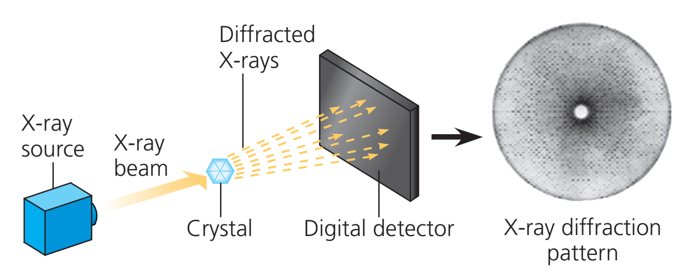
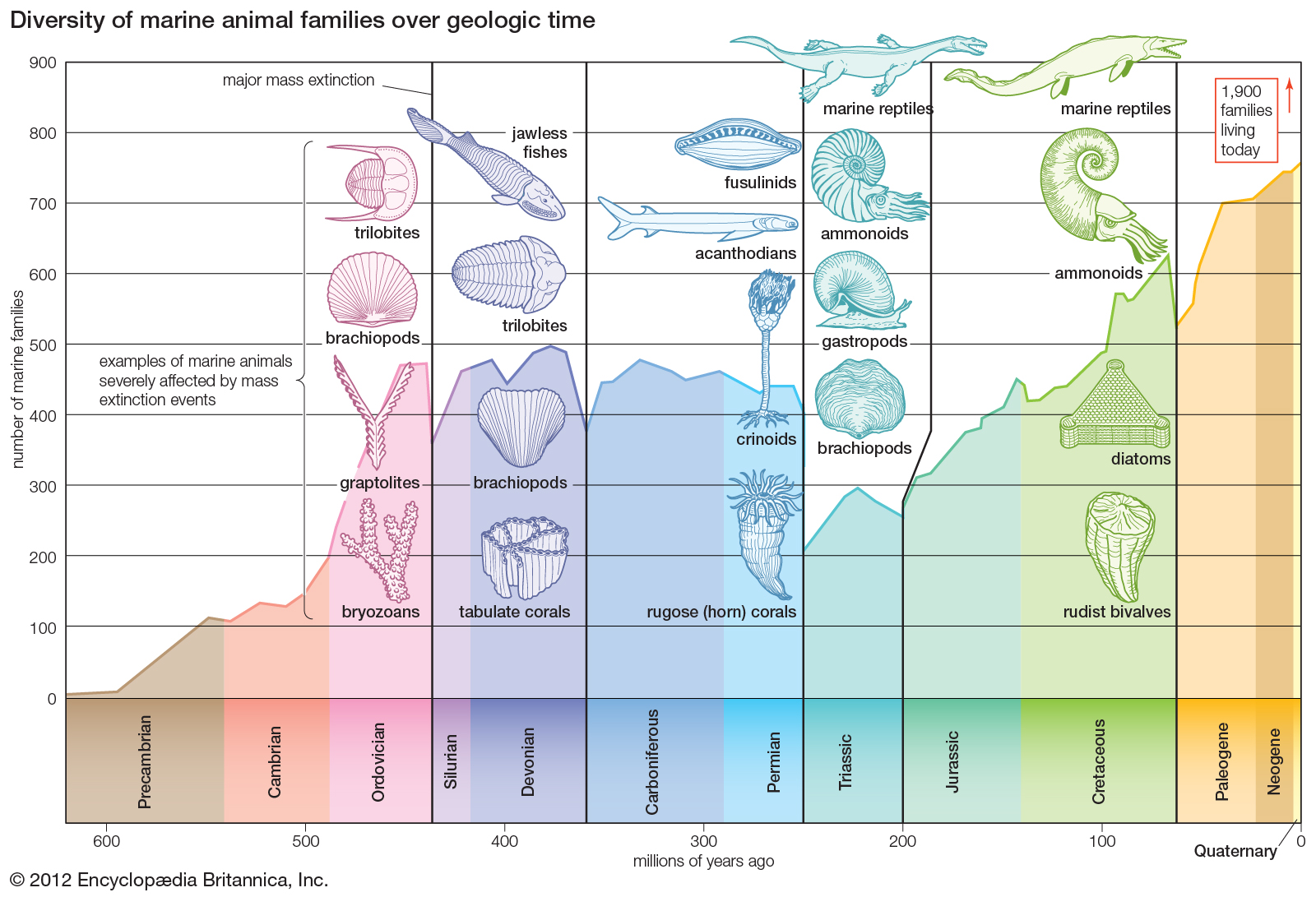
In a single-crystal X-ray diffraction measurement, a crystal is mounted on a goniometer. The goniometer is used to position the crystal at selected orientations. The crystal is illuminated with a finely focused monochromatic beam of X-rays, producing a diffraction pattern of regularly spaced spots known as reflections. The two-dimensional images taken at different orientations are converted into a three-dimensional model of the density of electrons within the crystal using the mathematical method of Fourier transforms, combined with chemical data known for the sample. Poor resolution (fuzziness) or even errors may result if the crystals are too small, or not uniform enough in their internal makeup.

X-ray crystallography is related to several other methods for determining atomic structures. Similar diffraction patterns can be produced by scattering electrons or neutrons, which are likewise interpreted by Fourier transformation. If single crystals of sufficient size cannot be obtained, various other X-ray methods can be applied to obtain less detailed information; such methods include fiber diffraction, powder diffraction and (if the sample is not crystallized) small-angle X-ray scattering (SAXS). If the material under investigation is only available in the form of nanocrystalline powders or suffers from poor crystallinity, the methods of electron crystallography can be applied for determining the atomic structure.

For all above mentioned X-ray diffraction methods, the scattering is elastic; the scattered X-rays have the same wavelength as the incoming X-ray. By contrast, inelastic X-ray scattering methods are useful in studying excitations of the sample such as plasmons, crystal-field and orbital excitations, magnons, and phonons, rather than the distribution of its atoms.

Workflow for solving the structure of a molecule by X-ray crystallography.

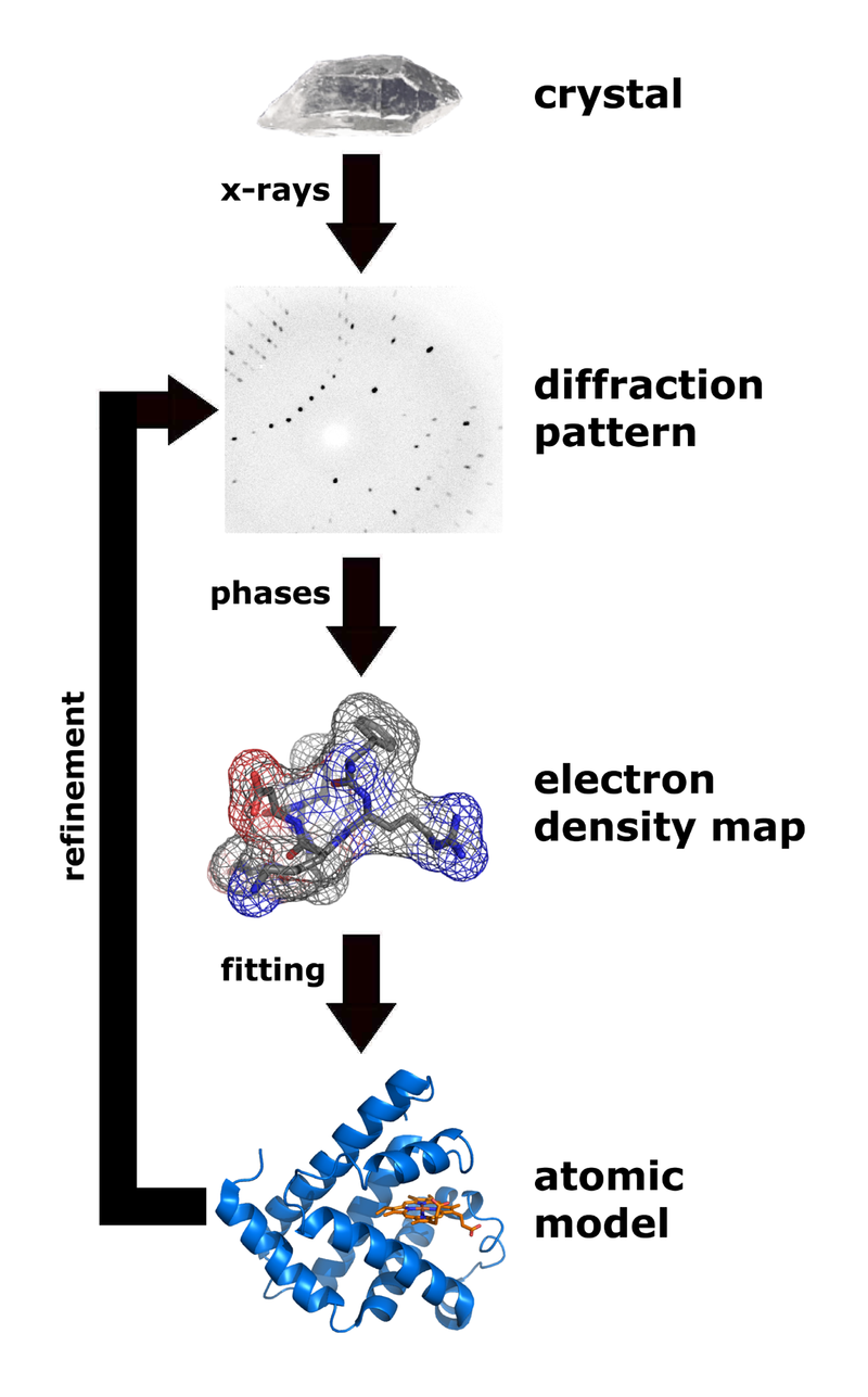
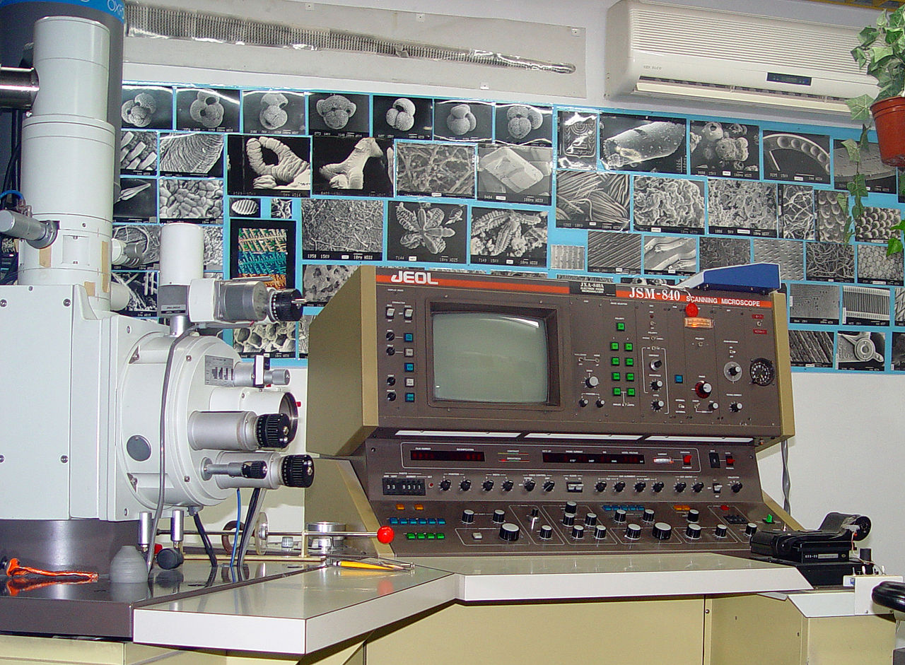
A powder x-ray diffractometer in motion.

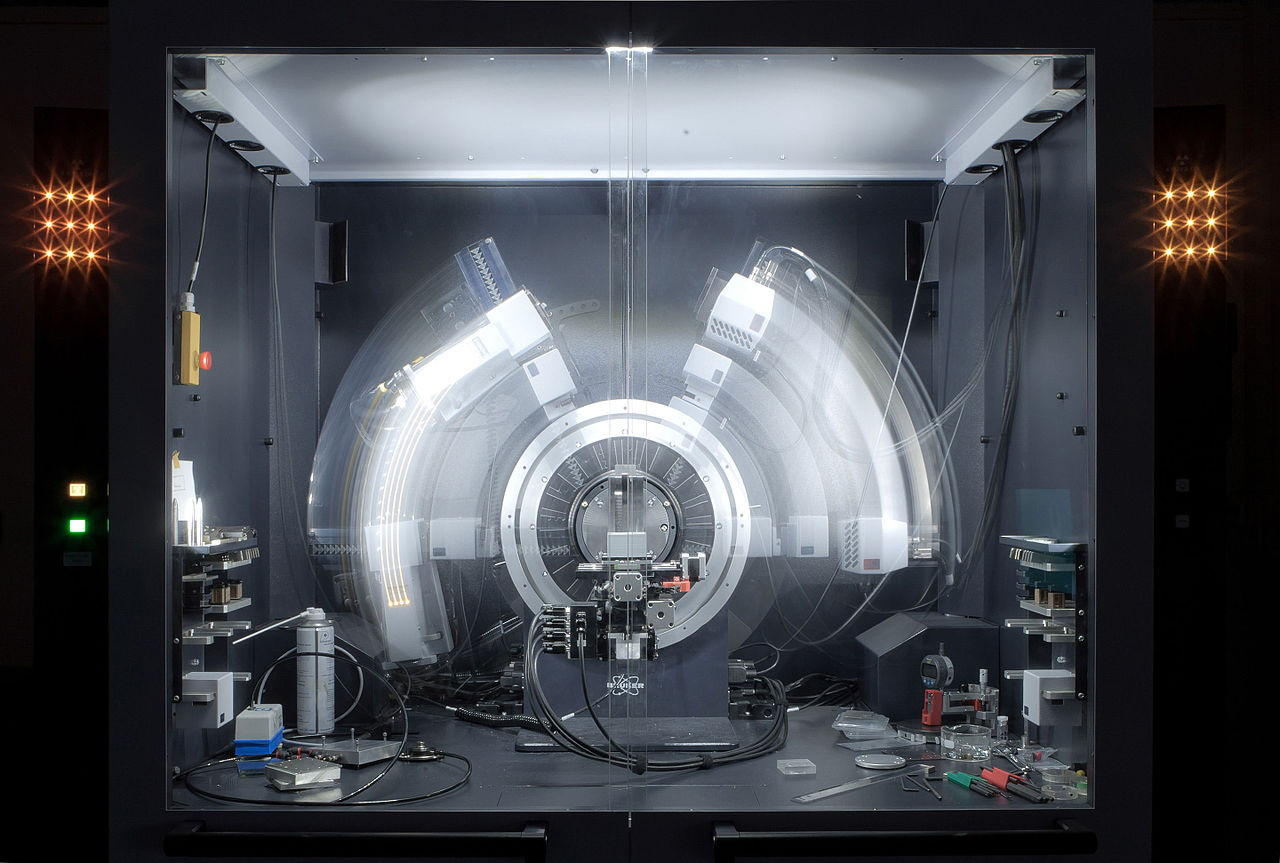
X-ray crystallography shows the arrangement of water molecules in ice, revealing the hydrogen bonds (1) that hold the solid together. Few other methods can determine the structure of matter with such precision (resolution).

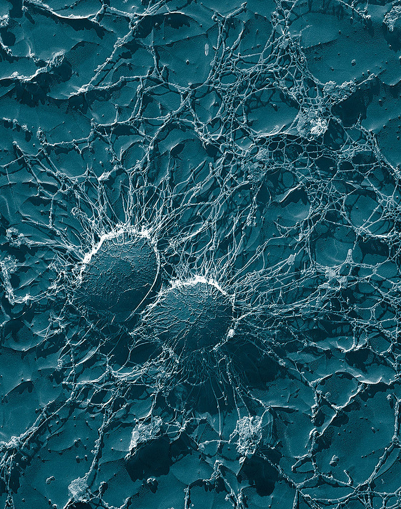
Crystal structures of proteins (which are irregular and hundreds of times larger than cholesterol) began to be solved in the late 1950s, beginning with the structure of sperm whale myoglobin by Sir John Cowdery Kendrew, for which he shared the Nobel Prize in Chemistry with Max Perutz in 1962. Since that success, over 130,000 X-ray crystal structures of proteins, nucleic acids and other biological molecules have been determined. The nearest competing method in number of structures analyzed is nuclear magnetic resonance (NMR) spectroscopy, which has resolved less than one tenth as many. Crystallography can solve structures of arbitrarily large molecules, whereas solution-state NMR is restricted to relatively small ones (less than 70 kDa). X-ray crystallography is used routinely to determine how a pharmaceutical drug interacts with its protein target and what changes might improve it. However, intrinsic membrane proteins remain challenging to crystallize because they require detergents or other denaturants to solubilize them in isolation, and such detergents often interfere with crystallization. Membrane proteins are a large component of the genome, and include many proteins of great physiological importance, such as ion channels and receptors. Helium cryogenics are used to prevent radiation damage in protein crystals.

On the other end of the size scale, even relatively small molecules may pose challenges for the resolving power of X-ray crystallography. The structure assigned in 1991 to the antibiotic isolated from a marine organism, diazonamide A (C₄₀H₃₄Cl₂N₆O₆, molar mass 765.65 g/mol), proved to be incorrect by the classical proof of structure: a synthetic sample was not identical to the natural product. The mistake was attributed to the inability of X-ray crystallography to distinguish between the correct -OH / -NH and the interchanged -NH₂ / -O- groups in the incorrect structure. With advances in instrumentation, however, similar groups can be distinguished using modern single-crystal X-ray diffractometers.

Despite being an invaluable tool in structural biology, protein crystallography carries some inherent problems in its methodology that hinder data interpretation. The crystal lattice, which is formed during the crystallization process, contains numerous units of the purified protein, which are densely and symmetrically packed in the crystal. When looking for a previously unknown protein, figuring out its shape and boundaries within the crystal lattice can be challenging. Proteins are usually composed of smaller subunits, and the task of distinguishing between the subunits and identifying the actual protein, can be challenging even for the experienced crystallographers. The non-biological interfaces that occur during crystallization are known as crystal-packing contacts (or simply, crystal contacts) and cannot be distinguished by crystallographic means. When a new protein structure is solved by X-ray crystallography and deposited in the Protein Data Bank, its authors are requested to specify the “biological assembly” which would constitute the functional, biologically-relevant protein. However, errors, missing data and inaccurate annotations during the submission of the data, give rise to obscure structures and compromise the reliability of the database. The error rate in the case of faulty annotations alone, has been reported to be upwards of 6,6% or approximately 15%, arguably a non-trivial size considering the number of deposited structures. This “interface classification problem” is typically tackled by computational approaches and has become a recognized subject in structural bioinformatics.